2 Example with opportunistic data on Dragonflies

In this example we are interested in exploring opportunistically collected data from the Swedish citizen science species observation portal - Artportalen.

2.1 Name searching

To begin with, we want be sure there is an unequivocal way to find the species within the order Odonata (dragonflies) and nothing else, so let’s search for “odonata”:

sx <- search_fulltext("odonata")
sx$data[, c("guid", "scientificName", "rank", "occurrenceCount")]

## [1] "https://species.biodiversitydata.se/ws/search.json?q=odonata&fq=idxtype%3ATAXON"

##       guid                          scientificName    rank occurrenceCount
## 1 10072832  Odonata associated gemycircularvirus 2 species               0
## 2  7367071    Ramalina fastigiata var. odonata Hue variety               0
## 3      789                                 Odonata   order           14121
## 4  8062407 Bdellodes odonata Wallace & Mahon, 1976 species               0
## 5  9829523  Odonata associated gemycircularvirus 1 species               0

We quickly see there that other taxonomic levels appear too, and also species that look suspiciously as not belonging to dragonflies. But there is only one order. Let’s refine the search. To know which search fields we can use to filter the search we use the function sbdi_fields(fields_type = "general"). The search field we are looking for is “order_s.”

sx <- search_fulltext(fq = "order_s:Odonata", page_size = 10)
sx$data[, c("scientificName", "rank", "occurrenceCount")]

## [1] "https://species.biodiversitydata.se/ws/search.json?fq=order_s%3AOdonata&fq=idxtype%3ATAXON&pageSize=10"

##        guid                        scientificName    rank occurrenceCount
## 1  11034676      Notoneura xanthe Lieftinck, 1938 species               0
## 2  11034731   Protoneura bifurcata Sjöstedt, 1918 species               0
## 3  11034937        Oxygomphus chapini Klots, 1944 species               0
## 4  11035128    Xerolestes pallidus (Rambur, 1842) species               0
## 5  11035335    Mesothemis mithroides Brauer, 1900 species               0
## 6  11029091 Paracercion luzonicum (Asahina, 1968) species               0
## 7  11029136         Onychargia stellata Ris, 1915 species               0
## 8  11029184         Nehalennia sophia Selys, 1840 species               0
## 9  11029206     Lestes lundquisti Lieftinck, 1949 species               0
## 10 11029310                Lestes concinnus Selys species               0

Now we can download the taxonomic data (note that the search is case-sensitive):

tx <- taxinfo_download("order_s:Odonata", 
                       fields = c("guid", "order_s","genus_s", "specificEpithet_s", 
                                  "scientificName",  "canonicalName_s", "rank"), 
                       verbose = FALSE)
tx <- tx[tx$rank == "species" & tx$genusS != "",] ## restrict to species and not hybrids

You can save the tx object as the complete species list for later use.

2.2 Filter the search to get the observations

We start by searching for the data resource we are interested in using the function pick_filter(). This is an interactive query guiding you through the many resources available to filtering your query (data resources, spatial layers, and curated species lists).

# follow the instructions 
fq_str <- pick_filter("resource") 

Follow the instructions. Your choices here would have been “in3” –> “dr5.” Your variable fq_str will now contain a string “data_resource_uid:dr5.”

We only want to look at data from year 2000 to 2010:

y1 <- 2000
y2 <- 2010
fq_str <- c(fq_str, paste0("year:[", y1, " TO ", y2,"]"))
# Note the square brackets are hard limits

We also want to filter spatially for Southern Sweden (Götaland).

Vector spatial layers (eg. polygons) can be imported in a number of different ways. SBDI APIs take as search input polygons in the so-called WKT Well Known Text format. So the first step is to load a vector layer and transform it into a WKT string. You could instead use the data we provid in the SBDI4R package data("swe").

data("swe",package = "SBDI4R")
wGotaland <- swe$Counties$LnNamn %in% c("Blekinge", "Gotlands", "Hallands", 
                                        "Jönköpings", "Kalmar", "Kronobergs", 
                                        "Östergötlands", "Skåne", "Västra Götalands")
gotaland_c <- swe$Counties[wGotaland,]

There are details about this polygon that we need to take care before. The WKT string should not be too long to be accepted by the API service. Also, the polygon we just got is projected in the coordinate system SWEREF99 TM, and the API service only accepts coordinates in a geodesic coordinate system WGS84. Let’s construct the WKT string:

# transform the CRS
gotaland_c <- st_transform(gotaland_c,
                           crs = st_crs(4326))

# disolve the counties into one polygon
gotaland <- st_union(gotaland_c)

# create a convex hull of the polygon to simplify the geometry and 
# reduce the length of the WKT string
gotaland_ch <- st_convex_hull(gotaland)

# cast it as MULTIPOLYGON as this is what SBDIs API need
# NOTE: as of today, the SBDI APIs will only work properly if the polygon is 
# submitted as a MULTIPOLYGON
gotaland_ch <- st_cast(gotaland_ch, to = "MULTIPOLYGON")

# create WKT string
wkt <- st_as_text(gotaland_ch)

The WKT string then looks like this:

## [1] "MULTIPOLYGON (((13.33575 55.34003, 12.81633 55.38594, 11.25342 58.35786, 11.13161 58.90942, 11.13145 59.01184, 11.21142 59.0897, 11.31566 59.11651, 11.82032 59.23553, 11.94833 59.26237, 12.06197 59.27159, 12.23104 59.27357, 15.79383 59.03876, 15.84306 59.02498, 19.2889 57.99043, 19.3058 57.96888, 18.90037 57.44014, 18.86704 57.39753, 18.3725 57.00678, 18.30044 56.9528, 16.40805 56.20229, 14.19057 55.38557, 13.33575 55.34003)))"

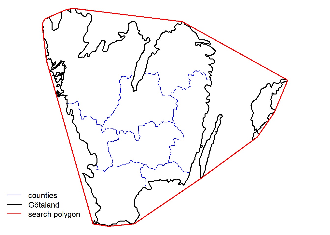
Next, we download the observations using the command occurrences(), but be aware that the search fields may not be the same as those used to search for taxa. We therefore recommend using the function sbdi_fields("occurrence") to find out which search fields we can use to filter for occurrences. Here we see that the field we need this time is “order.”

xf <- occurrences(taxon = "order:Odonata", 
                  fq = fq_str,
                  wkt = wkt,
                  extra = "collector",
                  email = "sbdi4r-test@biodiversitydata.se", 
                  download_reason_id = 10)

We have now downloaded the data locally and depending on your configuration this will be cached on your computer. However, as the search and download could take long time, we recommend to save the data locally. appropriate

save(xf, file = "an_appropriate_name.rdata")
load(file = "an_appropriate_name.rdata")

2.3 Quality and fit-for-use check

Before we can use the observation records we need to know if the observation effort (sampling effort) has varied over time and in space. We can approximate observation effort from the data by defining field visits i.e. occasions at which an observer has sampled observations. We reconstruct field visits (that is, assign each observation a visitUID) using using the package BIRDS. Additionally we want the data to be summarized over a grid of 25 km (provided through the SBDI4R package). The following functions will perform many different summaries at the same time. Please refer to the BIRDS package documentation for more detail.

remotes::install_github("GreenswayAB/BIRDS")
library(BIRDS)

OB <- organiseBirds(xf$data, sppCol = "species" , 
                    # We only want observations identified at the species level
                    taxonRankCol = "rank", taxonRank = "species", 
                    # the visits are defined by collector and named locality
                    idCols = c("locality", "collector"), 
                    timeCols = c("year", "month", "day"), 
                    xyCols = c("longitude","latitude") )

# We don't need the whole grid, just the piece that overlaps our searching polygon
wInt <- unlist(st_intersects(gotaland, Sweden_Grid_25km_Wgs84))
gotaland_grid25 <- Sweden_Grid_25km_Wgs84[wInt,]

SB <- summariseBirds(OB, grid = gotaland_grid25, spillOver = "unique")

Once summarised, we can see over space and for a few selected years how the number of observations is distributed:

maxC <- max(SB$spatial$nObs, na.rm = TRUE)
palBW <- leaflet::colorNumeric(c("white", "navyblue"), 
                               c(0, maxC), 
                               na.color = "transparent")
oldpar <- par()
par(mar = c(1,1,1,1), mfrow=c(1,3))
plot(SB$spatial$geometry, col=palBW(SB$spatial$nObs),
     border = "grey", main="All years") ## with palette
legend("bottomleft", inset = c(0,0.05),
       legend = round(seq(0, maxC, length.out = 5)),
       col = palBW(seq(0, maxC, length.out = 5)),
       title = "Number of \nobservations", pch = 15, bty="n")

## or export other combinations, e.g. one map per observed year
yearlySp <- exportBirds(SB, 
                        dimension = "spatial", 
                        timeRes = "yearly", 
                        variable = "nObs", 
                        method = "sum")

maxC <- max(yearlySp$'2005', na.rm = TRUE)
palBW <- leaflet::colorNumeric(c("white", "navyblue"), 
                               c(0, maxC), 
                               na.color = "transparent")

plot(yearlySp$geometry, col=palBW(yearlySp$'2005'), 
     border = "grey",main="2005")
legend("bottomleft", inset = c(0,0.05),
       legend = round(seq(0, maxC, length.out = 5)),
       col = palBW(seq(0, maxC, length.out = 5)),
       border = "grey",
       title = "Number of \nobservations", pch = 15, bty="n")

maxC <- max(yearlySp'2010', na.rm = TRUE)
palBW <- leaflet::colorNumeric(c("white", "navyblue"), 
                               c(0, maxC), 
                               na.color = "transparent")

plot(yearlySp$geometry, col=palBW(yearlySp$'2010'), 
     border = "grey",main="2010")
legend("bottomleft", inset = c(0,0.05),
       legend = round(seq(0, maxC, length.out = 5)),
       col = palBW(seq(0, maxC, length.out = 5)),
       border = "grey",
       title = "Number of \nobservations", pch = 15, bty="n")
par(oldpar)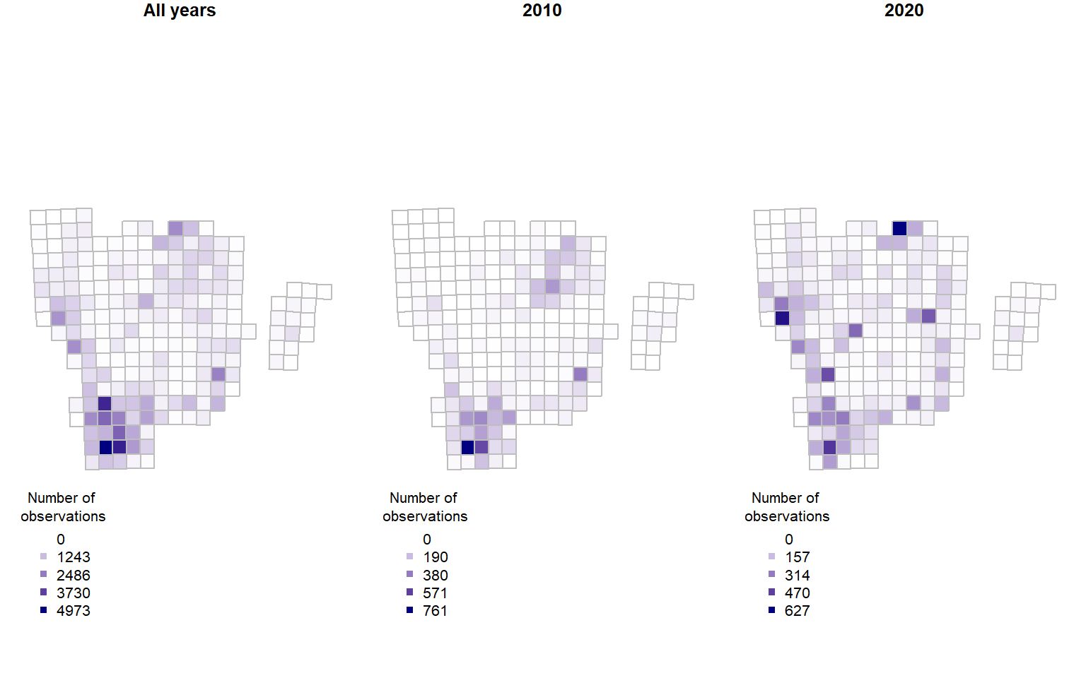

We now want to use the number of field visits as the measure for sampling effort. :

library(cowplot)
library(ggplot2)
library(colorRamps)
library(gridExtra)

vis <- ggplot(data = SB$spatial, aes( fill = nVis)) +
  geom_sf() +
  ggtitle("Visits") +
  scale_fill_gradient(low = "#56B1F7",
                      high = "#132B43",
                      na.value = NA) +
  theme(plot.margin = margin(1, 1, 1, 1, "pt")) +
  theme_cowplot()

spp <- ggplot(data = SB$spatial, aes( fill = nSpp)) +
  geom_sf() +
  ggtitle("Number of species") +
  scale_fill_gradient(low = "#56B1F7",
                      high = "#132B43",
                      na.value = NA) +
  theme(plot.margin = margin(1, 1, 1, 1, "pt")) +
  theme_cowplot()

grid.arrange(vis, spp, ncol = 2)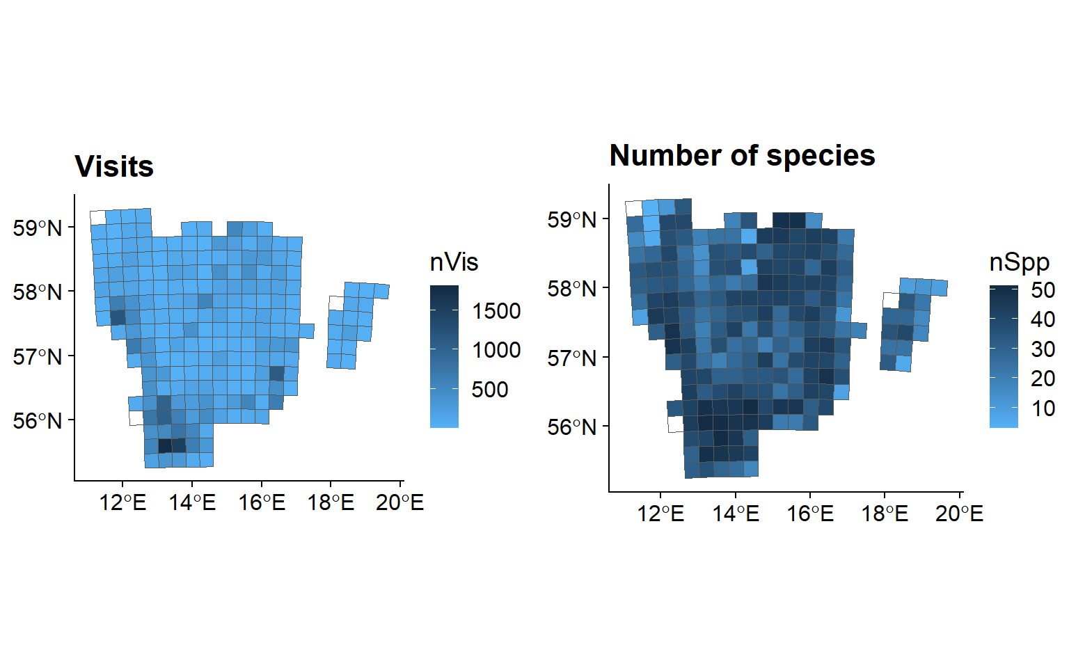

2.3.0.1 Temporal check

We see that SB contains an element called SB$temporal that contains a daily time series with time-specific rows when there is information. xts also supports day time, but dating below day resolution is not yet implemented in the BIRDS package.

sb.xts <- SB$temporal
head(sb.xts, 5)

##            nObs nVis nSpp
## 2000-03-24    1    1    1
## 2000-04-05    4    3    3
## 2000-04-06   11    6    3
## 2000-04-10    1    1    1
## 2000-04-12    3    3    1

Sub-setting is convenient in xts as you can do it with its dates and with a / for a range of dates.

sb.xts["2010-09-07"] #a specific day

##            nObs nVis nSpp
## 2010-09-07   19   10   12

sb.xts["2010-09-01/2010-09-15"] #for a period

##            nObs nVis nSpp
## 2010-09-01   46   19   14
## 2010-09-02   28   14   12
## 2010-09-03   23   10   10
## 2010-09-04   64   20   18
## 2010-09-05   74   27   12
## 2010-09-06   18    5   11
## 2010-09-07   19   10   12
## 2010-09-08   13    6    8
## 2010-09-09   32   12   14
## 2010-09-10    1    1    1
## 2010-09-11   16    9    8
## 2010-09-12   20   10    8
## 2010-09-13   14    5    9
## 2010-09-14    1    1    1
## 2010-09-15    3    3    2

sb.xts["2010-09"] #a specific month

##            nObs nVis nSpp
## 2010-09-01   46   19   14
## 2010-09-02   28   14   12
## 2010-09-03   23   10   10
## 2010-09-04   64   20   18
## 2010-09-05   74   27   12
## 2010-09-06   18    5   11
## 2010-09-07   19   10   12
## 2010-09-08   13    6    8
## 2010-09-09   32   12   14
## 2010-09-10    1    1    1
## 2010-09-11   16    9    8
## 2010-09-12   20   10    8
## 2010-09-13   14    5    9
## 2010-09-14    1    1    1
## 2010-09-15    3    3    2
## 2010-09-17    3    2    3
## 2010-09-18    9    5    5
## 2010-09-19   12    7    5
## 2010-09-21    3    2    3
## 2010-09-22    4    4    2
## 2010-09-23    3    3    2
## 2010-09-24   10    5    5
## 2010-09-25    7    4    6
## 2010-09-26    7    6    2
## 2010-09-28    2    2    2
## 2010-09-29    5    3    4
## 2010-09-30    2    2    2

The package xts has several tools for converting to different time periods. Here we use apply.monthly to obtain the total number of observations and visits per month. The plot command for an object of calss xts provides a many features. This makes it fairly easy to customize your plots. Read more in ?plot.xts.

library(xts)
obs.m <- apply.monthly(sb.xts$nObs, "sum", na.rm = TRUE)
vis.m <- apply.monthly(sb.xts$nVis, "sum", na.rm = TRUE)

plot(obs.m, 
     col = "darkblue", 
     grid.ticks.on = "month", 
     major.ticks = "year", 
     grid.col = "lightgrey",  
     main = "Total number of daily observations and visits per month")

lines(vis.m, col = "orange", lwd = 2, on = 1)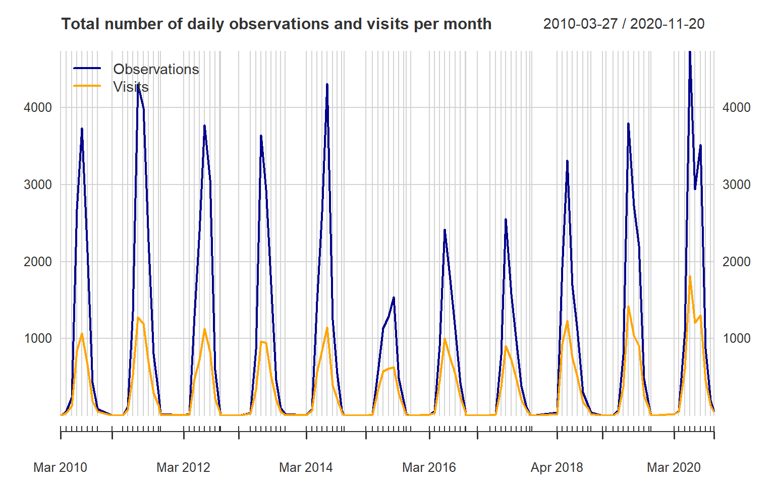

2.4 Species trends

We can now look at some particular species and ask whether those have changed in occurrence over time:

speciesSummary(SB)[,1:4]

##                       species nCells nObs nVis
## 1              Aeshna affinis      3   32   27
## 2             Aeshna caerulea      5   12   12
## 3               Aeshna cyanea    118  859  825
## 4              Aeshna grandis    145 1691 1661
## 5             Aeshna isoceles     14  102   99
## 6               Aeshna juncea     93  334  321
## 7                Aeshna mixta     72  645  614
## 8              Aeshna serrata     13   39   38
## 9           Aeshna subarctica     35  108   99
## 10             Aeshna viridis     13   40   35
## 11             Anax imperator     43  514  474
## 12            Anax parthenope      2    5    5
## 13        Brachytron pratense     82  434  421
## 14       Calopteryx splendens    101  681  627
## 15           Calopteryx virgo    122 1058 1004
## 16         Coenagrion armatum     23   74   67
## 17      Coenagrion hastulatum    116  930  897
## 18      Coenagrion johanssoni     15   75   70
## 19       Coenagrion lunulatum     42  111  104
## 20          Coenagrion puella    113 1313 1258
## 21      Coenagrion pulchellum    114 1364 1317
## 22     Cordulegaster boltonii     75  500  493
## 23             Cordulia aenea    116 1036 1017
## 24      Enallagma cyathigerum    138 1547 1461
## 25        Epitheca bimaculata     16   36   35
## 26           Erythromma najas     92  760  727
## 27       Erythromma viridulum     13  143  126
## 28      Gomphus vulgatissimus     48  160  155
## 29           Ischnura elegans    112 1210 1153
## 30           Ischnura pumilio     18   99   85
## 31               Lestes dryas     44  176  168
## 32              Lestes sponsa    137 1366 1295
## 33              Lestes virens     44  189  176
## 34     Leucorrhinia albifrons     40  143  138
## 35      Leucorrhinia caudalis     34  143  136
## 36         Leucorrhinia dubia     85  338  320
## 37    Leucorrhinia pectoralis     82  354  337
## 38     Leucorrhinia rubicunda     93  434  421
## 39         Libellula depressa    100  521  499
## 40            Libellula fulva      9  101   90
## 41   Libellula quadrimaculata    150 1971 1923
## 42        Nehalennia speciosa      3   34   33
## 43   Onychogomphus forcipatus     76  447  445
## 44      Orthetrum cancellatum    118  924  872
## 45     Orthetrum coerulescens     70  238  231
## 46       Platycnemis pennipes     91  544  528
## 47        Pyrrhosoma nymphula    124  967  938
## 48       Somatochlora arctica     28   45   42
## 49 Somatochlora flavomaculata     80  365  358
## 50     Somatochlora metallica    100  560  551
## 51             Sympecma fusca     40  179  174
## 52            Sympetrum danae    127  777  742
## 53        Sympetrum flaveolum     73  261  254
## 54     Sympetrum fonscolombii      2    2    2
## 55       Sympetrum sanguineum    124 1180 1136
## 56       Sympetrum striolatum     73  270  258
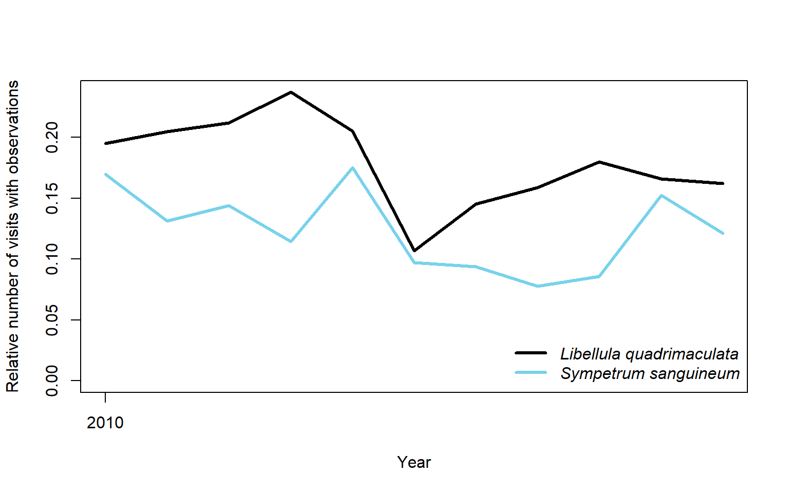
## 57         Sympetrum vulgatum    118 1028  972

We pick two species and compare their trends in number of visits where the species where reported, relative to the total number of visits.

library(dplyr)
sppCount <- obsData(OB) |> 
    group_by(year, visitUID) |> 
    summarise("focalCountLq" = sum(scientificName == "Libellula quadrimaculata"),
              "focalCountSd" = sum(scientificName == "Sympetrum sanguineum"),
              "sppLength" = length(unique(scientificName)), 
              .groups = "drop") |> 
    ungroup() |> 
    group_by(year) |> 
    summarise("focalCountLq" = sum(focalCountLq),
              "focalCountSd" = sum(focalCountSd),
              "nVis" = length(unique(visitUID)),
              "relCountLq" = focalCountLq / nVis,
              "relCountSd" = focalCountSd / nVis,
              .groups = NULL)

oldpar <- par(no.readonly = TRUE)
plot(sppCount$year, sppCount$relCountLq, 
     type = "l", lwd = 3, xlab = "Year", 
     ylab = "Relative number of visits with observations", 
     ylim = c(0, max(sppCount$relCountLq)), 
     xaxp = c(2000, 2010, 10))
lines(sppCount$year, sppCount$relCountSd, lwd = 3, col = "#78D2EB")
legend("bottomright", 
       legend = c("Libellula quadrimaculata","Sympetrum sanguineum"), 
       text.font = 3, col = c("black", "#78D2EB"), lwd = 3, bty = "n")

par(oldpar)