Here we provide a collection of use-examples showing a range of
queries that we think a typical use of the biodiversity infrastructure
may want to perform. sbdi4r2 is a wrapper for
galah customized to interact with the SDBI implementation.
galah is an R interface to biodiversity data hosted by the
‘living atlases’; a set of organisations that share a common codebase,
and act as nodes of the Global Biodiversity Information Facility (GBIF). These organisations collate and
store observations of individual life forms, using the ‘Darwin Core’ data standard.
The sbdi4r2 package is primarily for accessing data. It includes some filter functions that allow you to filter prior to download. It also includes (to be soon developed) some simple summary functions, and some functions for some simple data exploration. The examples also show you how you can use the data by exploring and analyzing with help of other R packages.
Please get in contact with us if you have questions regarding the use of the sbdi4r2 package.
Using sbdi4r2
Let’s assume you have already installed the package as shown in the main site.
Load the sbdi4r2 package:
library(sbdi4r2)
sbdi_config(email = "your.email@mail.com")
Then, check that we have some additional packages that we’ll use in the examples, and install them if necessary.
to_install <- c( "dplyr", "ggplot2", "htmlTable", "lubridate", "leaflet",
                 "maps", "mapdata", "phytools", "sf",  "tidyverse", "vegan")
to_install <- to_install[!sapply(to_install, requireNamespace, quietly = TRUE)]
if (length(to_install) > 0)
    install.packages(to_install, repos = "http://cran.us.r-project.org")
Example 1: Name searching and taxonomic trees

We want to look at the taxonomy of the Crested tit (Lophophanes cristatus), but we don’t know what the correct scientific name is, so let’s search for it:
sx <- sbdi_call() |>
sbdi_identify("parus") |>
atlas_species()
sx
#> # A tibble: 6 × 11
#> taxon_concept_id species_name scientific_name_auth…¹ taxon_rank kingdom phylum
#> <dbl> <chr> <chr> <chr> <chr> <chr>
#> 1 9705453 Parus major Linnaeus, 1758 species Animal… Chord…
#> 2 4409010 Parus monta… Conrad von Baldenstei… species Animal… Chord…
#> 3 2487931 Parus afer Gmelin, 1789 species Animal… Chord…
#> 4 2487941 Parus niger Vieillot, 1818 species Animal… Chord…
#> 5 2487926 Parus rufiv… Bocage, 1877 species Animal… Chord…
#> 6 2487946 Parus grise… Reichenow, 1882 species Animal… Chord…
#> # ℹ abbreviated name: ¹scientific_name_authorship
#> # ℹ 5 more variables: class <chr>, order <chr>, family <chr>, genus <chr>,
#> # vernacular_name <chr>But we see that some non-birds are also returned, e.g. insects
(Neuroctenus parus). We want to restrict the search to the
family Paridae, but filter out hybrids between genus
(genus == NA).
sx <- sbdi_call() |>
        sbdi_identify("paridae") |>
        atlas_species() |>
        filter(!is.na(genus)) |>
        as.data.frame()
sx
#>    taxon_concept_id                 species_name     scientific_name_authorship
#> 1           9705453                  Parus major                 Linnaeus, 1758
#> 2           2487879          Cyanistes caeruleus               (Linnaeus, 1758)
#> 3           2487843            Poecile palustris               (Linnaeus, 1758)
#> 4           2487871               Periparus ater               (Linnaeus, 1758)
#> 5           2487866             Poecile montanus (Conrad von Baldenstein, 1827)
#> 6           2487883        Lophophanes cristatus               (Linnaeus, 1758)
#> 7           2487862              Poecile cinctus               (Boddaert, 1783)
#> 8          10525787 Cyanistes cyanus x caeruleus                           <NA>
#> 9           2487877             Cyanistes cyanus                 (Pallas, 1770)
#> 10          4409010               Parus montanus   Conrad von Baldenstein, 1827
#> 11          2487805         Poecile atricapillus               (Linnaeus, 1766)
#> 12         10308870   Poecile cinctus x montanus                           <NA>
#> 13          2487931                   Parus afer                   Gmelin, 1789
#> 14          2487941                  Parus niger                 Vieillot, 1818
#> 15          2487793           Poecile hudsonicus            (J.R.Forster, 1772)
#> 16          2487857             Poecile lugubris               (Temminck, 1820)
#> 17          2487887           Baeolophus bicolor               (Linnaeus, 1766)
#> 18          2487926            Parus rufiventris                   Bocage, 1877
#> 19          2487946          Parus griseiventris                Reichenow, 1882
#>    taxon_rank  kingdom   phylum class         order  family       genus
#> 1     species Animalia Chordata  Aves Passeriformes Paridae       Parus
#> 2     species Animalia Chordata  Aves Passeriformes Paridae   Cyanistes
#> 3     species Animalia Chordata  Aves Passeriformes Paridae     Poecile
#> 4     species Animalia Chordata  Aves Passeriformes Paridae   Periparus
#> 5     species Animalia Chordata  Aves Passeriformes Paridae     Poecile
#> 6     species Animalia Chordata  Aves Passeriformes Paridae Lophophanes
#> 7     species Animalia Chordata  Aves Passeriformes Paridae     Poecile
#> 8     species Animalia Chordata  Aves Passeriformes Paridae   Cyanistes
#> 9     species Animalia Chordata  Aves Passeriformes Paridae   Cyanistes
#> 10    species Animalia Chordata  Aves Passeriformes Paridae       Parus
#> 11    species Animalia Chordata  Aves Passeriformes Paridae     Poecile
#> 12    species Animalia Chordata  Aves Passeriformes Paridae     Poecile
#> 13    species Animalia Chordata  Aves Passeriformes Paridae       Parus
#> 14    species Animalia Chordata  Aves Passeriformes Paridae       Parus
#> 15    species Animalia Chordata  Aves Passeriformes Paridae     Poecile
#> 16    species Animalia Chordata  Aves Passeriformes Paridae     Poecile
#> 17    species Animalia Chordata  Aves Passeriformes Paridae  Baeolophus
#> 18    species Animalia Chordata  Aves Passeriformes Paridae       Parus
#> 19    species Animalia Chordata  Aves Passeriformes Paridae       Parus
#>                       vernacular_name
#> 1                           Great Tit
#> 2                   Eurasian Blue Tit
#> 3                           Marsh Tit
#> 4                            Coal Tit
#> 5                          Willow Tit
#> 6                         Crested Tit
#> 7               Gray-headed Chickadee
#> 8                Azure Tit x Blue Tit
#> 9                           Azure Tit
#> 10                         willow tit
#> 11             Black-Capped Chickadee
#> 12 Grey-headed Chickadee x Willow Tit
#> 13                           Gray Tit
#> 14                 Southern Black-Tit
#> 15                   Boreal Chickadee
#> 16                         Sombre Tit
#> 17                 Sennett'S Titmouse
#> 18                 Rufous-bellied Tit
#> 19                         Miombo Tit
Do you find it?
We can make a taxonomic tree plot using the phytools
package:
library(phytools)
## as.phylo requires the taxonomic columns to be factors
sx$genus <- as.factor(sx$genus)
sx$species_name <- as.factor(sx$species_name)
sx$vernacular_name <- as.factor(sx$vernacular_name)

## create phylo object of canonical name nested within Genus
ax <- as.phylo(~genus/species_name, data = sx)
plotTree(ax, fsize = 0.7, ftype="i") ## plot it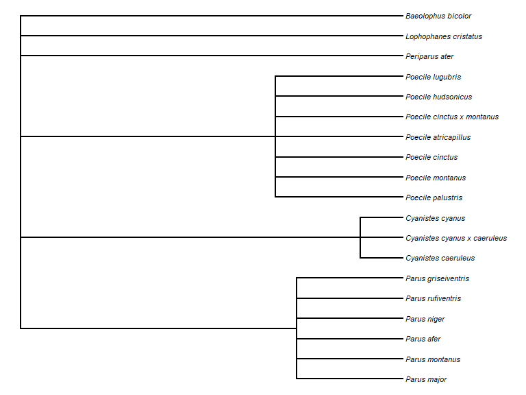
Example 2: Get some data and work it out
Let’s filter, get quality assertions, plot data on a map and save it. First let’s download occurrence data for the “Sommarlånke” and view top of the data table:
library(dplyr)
#>
#> Attaching package: 'dplyr'
#> The following object is masked from 'package:galah':
#>
#>     desc
#> The following objects are masked from 'package:stats':
#>
#>     filter, lag
#> The following objects are masked from 'package:base':
#>
#>     intersect, setdiff, setequal, union
library(htmlTable)

focal_spp <- search_taxa("Callitriche cophocarpa")
## or equally valid
focal_spp <- search_taxa("sommarlånke")
focal_spp$taxon_concept_id
#> [1] "8236752"

x <- sbdi_call() |>
  sbdi_identify("Callitriche cophocarpa") |>
  atlas_occurrences()
#> Request for 614 occurrences placed in queue
#> Current queue length: 1
#> Downloading

x |>
  pull(dataResourceName) |>
  table() |>
  as.data.frame() |>
  rename("Source" = Var1) |>
htmlTable()| Source | Freq | |
|---|---|---|
| 1 | Herbarium GB, University of Gothenburg | 2 |
| 2 | Lund University Biological Museum - Botanical collection (LD) | 384 |
| 3 | National Wetland Inventory (NV) | 15 |
| 4 | Oskarshamn herbarium (OHN) | 211 |
| 5 | SHARK - Regional marine environmental monitoring and monitoring projects of Epibenthos in Sweden since 1994 | 2 |
You can also search for a set of species simultaneously.
taxa <- c("Callitriche", "Anarrhinum")
x <- sbdi_call() |>
  sbdi_identify(taxa) |>
  atlas_occurrences()
#> --

x |>
  pull(dataResourceName) |>
  table() |>
  as.data.frame() |>
  rename("Source" = Var1) |>
htmlTable()| Source | Freq | |
|---|---|---|
| 1 | Artportalen (Swedish Species Observation System) | 21330 |
| 2 | Botany (UPS) | 487 |
| 3 | Herbarium GB, University of Gothenburg | 17 |
| 4 | Lund University Biological Museum - Botanical collection (LD) | 2156 |
| 5 | National Wetland Inventory (NV) | 89 |
| 6 | Oskarshamn herbarium (OHN) | 776 |
| 7 | Phanerogamic Botanical Collections (S) | 2628 |
| 8 | SHARK - National marine environmental monitoring of Epibenthos in Sweden since 1992 | 56 |
| 9 | SHARK - Regional marine environmental monitoring and monitoring projects of Epibenthos in Sweden since 1994 | 2309 |
| 10 | The Bergius Herbarium | 1 |
Search filters
There are different data sources. Let’s assume you only need to see data from one source, e.g. Lund University Biological Museum - Botanical collection (LD), which we just happen to know its UID is “dr2” (more about how to find out this later):
taxa <- "Callitriche cophocarpa"
xf <- sbdi_call() |>
  sbdi_identify(taxa) |>
  filter(dataResourceUid == "dr2") |>
  atlas_occurrences()

xf |>
  pull(dataResourceName) |>
  table() |>
  as.data.frame() |>
  rename("Source" = Var1) |>
htmlTable()| Source | Freq | |
|---|---|---|
| 1 | Lund University Biological Museum - Botanical collection (LD) | 384 |
What to search for?
The package offers a function show_all_fields() to help
you know what fields you can query. There are many such help functions,
check ?show_all().
show_all(fields)For example, in SBDI all fields starting with “cl” are spatial layers.
show_all(fields) |>
  filter(grepl("cl", id)) |>
  as.data.frame() |>
  head(10)
#>         id                         description   type
#> 1  cl10038             Sweden-Country Boundary fields
#> 2  cl10040                            Kommuner fields
#> 3  cl10041                         FA-regioner fields
#> 4  cl10042                         LA-regioner fields
#> 5  cl10046                               Sjöar fields
#> 6  cl10047                          Kustvatten fields
#> 7  cl10048                         Grundvatten fields
#> 8  cl10050    Nyckelbiotoper - Storskogsbruket fields
#> 9  cl10051              Gräns för contortatall fields
#> 10 cl10052 Terrestrial Ecoregions of the World fields
You can use the spatial layers that are available to spatially search for the indexed observations.
show_all(fields) |>
  filter(description == "Län") |>
  as.data.frame()

xf <- sbdi_call() |>
  sbdi_identify(taxa) |>
  filter("cl10097" == "Uppsala") |>
  atlas_occurrences()
Note that this is fundamentally different than filtering by
county=Uppsala as this will search for the text
Uppsala in the field county, rather than
spatially matching the observations.
[TO BE DEVELOPED] Otherwise, you can search available data resources,
collections (and more) using the interactive function
pick_filter. The pick_filter function lets you
explore data collections, spatial layers. Soon there will be more
indexed fields.
Any search could be filtered by any indexed field (a.k.a. column or variable). For example, let’s filter observations with coordinate uncertainty smaller than or equal to 100 m.
xf <- sbdi_call() |>
  sbdi_identify(taxa) |>
  filter(coordinateUncertaintyInMeters <= 100) |>
  atlas_occurrences()
One could search for observations in specific years:
x2yr <- sbdi_call() |>
  sbdi_identify(taxa) |>
  filter(year == 2010 | year == 2020) |>
  atlas_occurrences()
In the same way, one could search for observations between two years:
library(lubridate)
xf <- sbdi_call() |>
  sbdi_identify(taxa) |>
  filter(year >= 2010, year <= 2020) |>
  atlas_occurrences()
Likewise, search conditions can be accumulated and will be treated as AND conditions:
or, occurrences could be filtered by the basis of record (that is, how was the observation recorded):
xbor <- sbdi_call() |>
  sbdi_identify(taxa) |>
  filter(basisOfRecord == "PreservedSpecimen") |>
  select(basisOfRecord, group = "basic") |>
  atlas_occurrences()
In this last example we introduce the use of select(). This function
will control which columns you retrieve from the atlas. By default, a
minimum set of columns is pre-selected. But any field you can search for
can be retrieved. See more about this function
?sbdi_select()
Quality assertions
Data quality assertions are a suite of fields that are the result of a set of tests performed on data. We continue using the data for the Blunt-fruited Water-starwort and get a summary of the data quality assertions,
You can see a list of all record issues using
show_all(assertions) and see what is considered as fatal
quality issues, that is category = “Error” or “Warning”.
show_all(assertions)
#> # A tibble: 114 × 4
#>    id                                 description                 category type
#>    <chr>                              <chr>                       <chr>    <chr>
#>  1 AMBIGUOUS_COLLECTION               Ambiguous collection        Warning  asse…
#>  2 AMBIGUOUS_INSTITUTION              Ambiguous institution       Warning  asse…
#>  3 BASIS_OF_RECORD_INVALID            Basis of record badly form… Warning  asse…
#>  4 biosecurityIssue                   Biosecurity issue           Error    asse…
#>  5 COLLECTION_MATCH_FUZZY             Collection match fuzzy      Warning  asse…
#>  6 COLLECTION_MATCH_NONE              Collection not matched      Warning  asse…
#>  7 CONTINENT_COUNTRY_MISMATCH         Continent country mismatch  Warning  asse…
#>  8 CONTINENT_DERIVED_FROM_COORDINATES Continent derived from coo… Warning  asse…
#>  9 CONTINENT_INVALID                  Continent invalid           Warning  asse…
#> 10 COORDINATE_INVALID                 Coordinate invalid          Warning  asse…
#> # ℹ 104 more rows
search_all(assertions, "longitude")
#> # A tibble: 2 × 4
#>   id                             description                      category type
#>   <chr>                          <chr>                            <chr>    <chr>
#> 1 PRESUMED_NEGATED_LONGITUDE     Longitude is negated             Warning  asse…
#> 2 COORDINATE_REPROJECTION_FAILED Decimal latitude/longitude conv… Warning  asse…

assertError <- show_all(assertions) |>
  filter(category == "Error")

xassert <- sbdi_call() |>
  sbdi_identify(taxa) |>
  select(assertError$id, group = "basic") |>
  atlas_occurrences()
#> Request for 614 occurrences placed in queue
#> Current queue length: 1
#> Downloading

assert_count <- colSums(xassert[,assertError$id])
assert_count
#>                biosecurityIssue                 detectedOutlier
#>                               0                               0
#>                 habitatMismatch         identificationIncorrect
#>                               0                               0
#>            INTERPRETATION_ERROR      SENSITIVITY_REPORT_INVALID
#>                               0                               0
#> SENSITIVITY_REPORT_NOT_LOADABLE                  taxonomicIssue
#>                               0                               0
#>                   temporalIssue    UNRECOGNISED_COLLECTION_CODE
#>                               0                               0
#>   UNRECOGNISED_INSTITUTION_CODE              userAssertionOther
#>                               0                               0

assertWarning <- show_all(assertions) |>
  filter(category == "Warning")

xassert <- sbdi_call() |>
  sbdi_identify(taxa) |>
  select(all_of(assertWarning$id), group = "basic") |>
  atlas_occurrences()
#> Request for 614 occurrences placed in queue
#> Current queue length: 1
#> -
#> Downloading

assert_count <- colSums(xassert[,assertWarning$id])
assert_count[which(assert_count > 0)]
#>                     COORDINATE_PRECISION_INVALID
#>                                              122
#>            COORDINATE_UNCERTAINTY_METERS_INVALID
#>                                              404
#>                      COUNTRY_COORDINATE_MISMATCH
#>                                                1
#>                 COUNTRY_DERIVED_FROM_COORDINATES
#>                                                2
#>                                   FIRST_OF_MONTH
#>                                               19
#>                            LOCATION_NOT_SUPPLIED
#>                                               13
#>                          MISSING_COLLECTION_DATE
#>                                               23
#>                            MISSING_GEODETICDATUM
#>                                              599
#>                        MISSING_GEOREFERENCE_DATE
#>                                              614
#>                          MISSING_GEOREFERENCEDBY
#>                                              614
#>                     MISSING_GEOREFERENCEPROTOCOL
#>                                              614
#>                      MISSING_GEOREFERENCESOURCES
#>                                              614
#>                                MISSING_TAXONRANK
#>                                              612
#>  OCCURRENCE_STATUS_INFERRED_FROM_BASIS_OF_RECORD
#>                                                2
#> OCCURRENCE_STATUS_INFERRED_FROM_INDIVIDUAL_COUNT
#>                                              384
#>                            RECORDED_DATE_INVALID
#>                                                2
#>                        STATE_COORDINATE_MISMATCH
#>                                              335
#>                         UNCERTAINTY_IN_PRECISION
#>                                              122
Plotting data on a map
xf <- sbdi_call() |>
  sbdi_identify(taxa) |>
  atlas_occurrences()

  data("swe_wgs84", package = "sbdi4r2", envir = environment())
plot(swe_wgs84[["Border"]]$geometry, col = "grey", border = NA)
  points(xf$decimalLongitude, xf$decimalLatitude, pch = 19, col = "black")
There are many other ways of producing spatial plots in R, for
example using the package sf.
library(sf)

xf_sf <- xf |>
  filter(!is.na(decimalLatitude),
         !is.na(decimalLongitude)) |>
  st_as_sf(coords = c("decimalLongitude", "decimalLatitude"),
           crs = 4326)
plot(swe_wgs84[["Border"]]$geometry, col = "grey", border = NA)
plot(xf_sf$geometry, pch = 19, add = TRUE)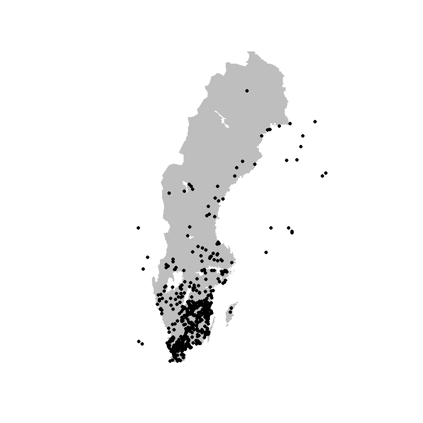
The leaflet package provides a simple method of
producing browser-based maps with panning, zooming, and background
layers:
library(leaflet)
## make a link to the web page for each occurrence
popup_link <- paste0("<a href=\"https://records.biodiversitydata.se/occurrences/",
                      xf_sf$recordID,"\">Link to occurrence record</a>")

## blank map, with imagery background
m <- leaflet() |>
  addProviderTiles("Esri.WorldImagery") |>
  addCircleMarkers(data = xf_sf ,
                   radius = 2, fillOpacity = .5, opacity = 1,
                   popup = popup_link)
mSave the data
# save as data.frame
Callitriche <- as.data.frame(xf)

# simplyfy data frame
calli <- data.frame(Callitriche$scientificName,
                    Callitriche$decimalLatitude,
                    Callitriche$decimalLongitude)
# simplify column names
colnames(calli) <- c("species","latitude","longitude")
# remove rows with missing values (NAs)
calli <- na.omit(calli)

# save as csv
write.csv(calli, "Callitriche.csv")

# save as R specific format rds
saveRDS(calli, "Callitriche.rds")
Example 3: Summarise occurrences over a defined grid
Now, following with the data downloaded in the previous example, we want to summarise occurrences over a defined grid instead of plotting every observation point. First we need to overlay the observations with the grid. In this case, the standard Swedish grids at 50, 25, 10 and 5 km are provided as data (with Coordinate Reference System WGS84 EPSG:4326).
# load some shapes over Sweden
# Political borders
data("swe_wgs84", package = "sbdi4r2", envir = environment())
# A standard 50km grid
data("Sweden_Grid_50km_Wgs84", package = "sbdi4r2", envir = environment())

grid <- Sweden_Grid_50km_Wgs84

## overlay the data with the grid
listGrid <- st_intersects(grid, xf_sf)

ObsInGridList <- list()
for (i in seq(length(listGrid))) {
  if (length(listGrid[[i]]) == 0) {
    ObsInGridList[[i]] <- NA
  } else {
    ObsInGridList[[i]] <- st_drop_geometry(xf_sf[listGrid[[i]],])
  }
}

wNonEmpty <- which( unlist(lapply(ObsInGridList, function(x) !all(is.na(x)))) )
if (length(wNonEmpty) == 0) message("Observations don't overlap any grid cell.")

## a simple check of number of observations
nObs <- nrow(xf_sf)
sum(unlist(lapply(ObsInGridList, nrow))) == nObs
#> [1] FALSE
The result ObsInGridList is a list object
with a subset of the data on each grid.
Summarise
Now let’s summarise occurrences within grid cells:
## apply a summary over the grid
nCells <- length(ObsInGridList)

res <- data.frame("nObs" = as.numeric(rep(NA, nCells)),
                  "nYears" = as.numeric(rep(NA, nCells)),
                  row.names = row.names(grid),
                  stringsAsFactors = FALSE)

cols2use <- c("scientificName", "eventDate")

dataRes <- lapply(ObsInGridList[wNonEmpty], function(x){
  x <- x[,cols2use]
  x$year <- year(x$eventDate)
  colnames(x) <- c("scientificName", "year")

  return(c("nObs" = nrow(x),
           "nYears" = length(unique(x[,"year"]))
  ))
})

dataRes <- as.data.frame(dplyr::bind_rows(dataRes, .id = "id"))

res[wNonEmpty,] <- dataRes[,-1]
res$nObs <- as.numeric(res$nObs)
resSf <- st_as_sf(cbind(res, st_geometry(grid)) )
rownames(resSf) <- grid$id
Plotting data on a map
Finally plot the grid summary as a map:
palBW <- leaflet::colorNumeric(palette = c("white", "navyblue"),
                               domain = c(0, max(resSf$nObs, na.rm = TRUE)),
                               na.color = "transparent")
oldpar <- par()
par(mar = c(1,1,0,0))
plot(resSf$geometry, col = palBW(resSf$nObs), border = NA)
plot(swe_wgs84$Border, border = 1, lwd = 1, add = T)
legend("bottomleft",
       legend = round(seq(0, max(resSf$nObs, na.rm = TRUE), length.out = 5)),
       col = palBW(seq(0, max(resSf$nObs, na.rm = TRUE), length.out = 5)),
       title = "Number of \nobservations", pch = 15, bty = "n")
suppressWarnings(par(oldpar))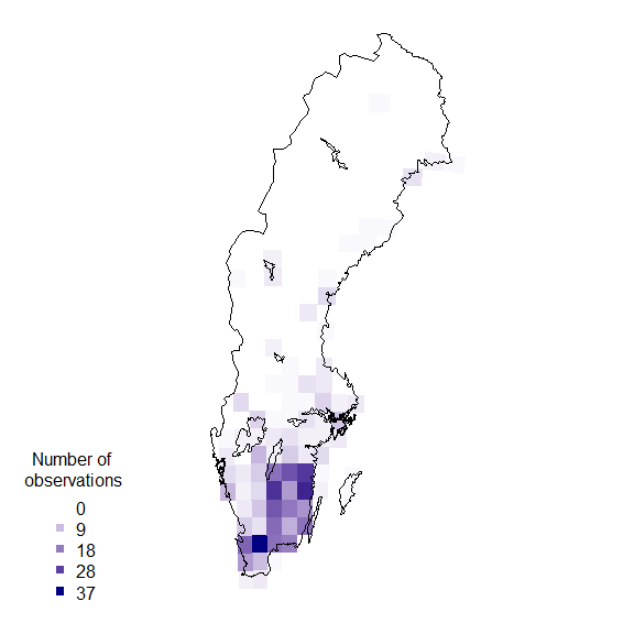
Other polygons
Any other set of polygons could also be used to summarise, for example, the counties.
counties <- swe_wgs84$Counties
obs <- st_transform(xf_sf, crs = st_crs(counties))

## overlay the data with the counties
listGrid <- st_intersects(counties, obs)

ObsInCountyList <- list()
for (i in seq(length(listGrid))) {
  if (length(listGrid[[i]]) == 0) {
    ObsInCountyList[[i]] <- NA
  } else {
    ObsInCountyList[[i]] <- st_drop_geometry(xf_sf[listGrid[[i]],])
  }
}
wNonEmpty <- which( unlist(lapply(ObsInCountyList, function(x) !all(is.na(x)))) )
if (length(wNonEmpty) == 0) message("Observations don't overlap any grid cell.")

## check nObs
sum(unlist(lapply(ObsInCountyList, nrow))) == nObs # some observations are not in the counties territory
#> [1] FALSE
length(ObsInCountyList) == nrow(counties)
#> [1] TRUE

## apply a summary over the grid
nCells <- length(ObsInCountyList)

res <- data.frame("nObs" = as.numeric(rep(NA, nCells)),
                  "nYears" = as.numeric(rep(NA, nCells)),
                  stringsAsFactors = FALSE)

cols2use <- c("scientificName", "eventDate")

dataRes <- lapply(ObsInCountyList[wNonEmpty], function(x){
  x <- x[,cols2use]
  x$year <- year(x$eventDate)
  colnames(x) <- c("scientificName", "year")

  return(c("nObs" = nrow(x),
           "nYears" = length(unique(x[,"year"]))
  ))
})

dataRes <- as.data.frame(dplyr::bind_rows(dataRes, .id = "id"))
res[wNonEmpty,] <- dataRes[,-1]
res$nObs <- as.numeric(res$nObs)

resSf <- st_as_sf(cbind(res, st_geometry(counties)))
rownames(resSf) <- counties$LnNamn
and again plotting as a map:
palBW <- leaflet::colorNumeric(c("white", "navyblue"),
                               c(0, max(resSf$nObs, na.rm = TRUE)),
                               na.color = "transparent")
oldpar <- par()
par(mar = c(1,1,0,0))
plot(resSf$geometry, col = palBW(resSf$nObs), border = NA)
plot(swe_wgs84$Border, border = 1, lwd = 1, add = T)
text(st_coordinates(st_centroid(counties)),
    labels = as.character(counties$LnNamn), font = 2, cex = .5 )
legend("bottomleft",
       legend = round(seq(0, max(resSf$nObs, na.rm = TRUE), length.out = 5)),
       col = palBW(seq(0, max(resSf$nObs, na.rm = TRUE), length.out = 5)),
       title = "Number of \nobservations", pch = 15, bty = "n")
suppressWarnings(par(oldpar))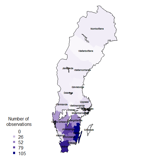
Add the county name to each observation
Let’s try adding a column to the observations data frame to hold the id of the overlapped polygon, in this case, Län (county) and plot which observation didn’t fall with any county.
countiesLab <- as.character(counties$LnNamn)
obs$county <- countiesLab[as.integer(st_intersects(obs, counties))]

oldpar <- par()
par(mar = c(1,1,0,0))
plot(counties$geometry, border = 1, lwd = 1)
plot(obs$geometry[which(is.na(obs$county))],
     pch = 19, cex = .5, col = "red", add = T)
suppressWarnings(par(oldpar))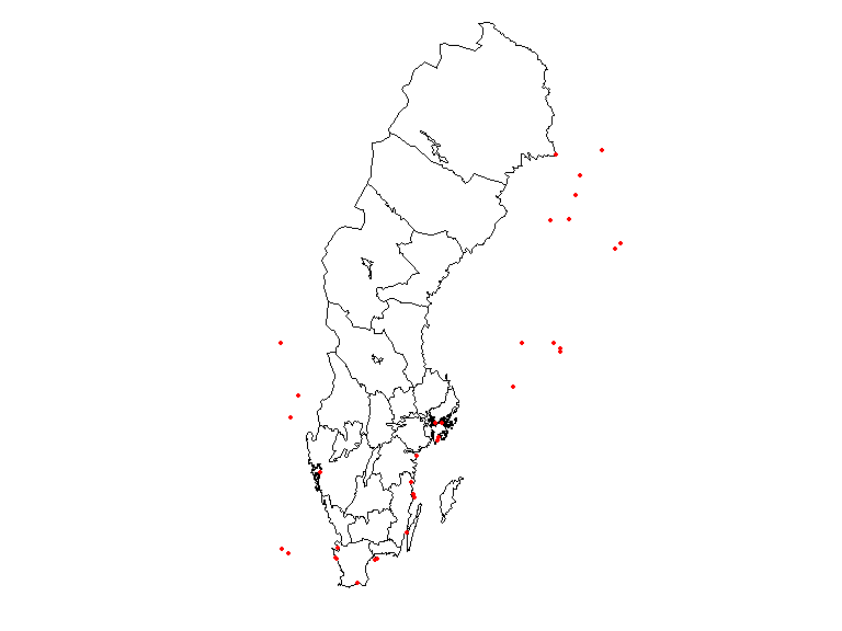
It is clear from this image that there are observations outside the territorial extent of the country but that may be within coastal areas or reported by a Swedish institution outside the country.
Example 4: Area search and report.
Let’s now ask: Which listed species of amphibians were observed in a Örebro?
Vector spatial layers (eg. polygons) can be imported in a number of
different ways and the package helps to pass those polygons into the
search. So the first step is to load a vector spatial layer. Download a
.zip file with different delimitation
for Sweden and move it somewhere you like in your computer. We
recommend you move it into your working directory
(getwd()). Extract the .zip file named
KommunSweref99.zip.
This will only work when you set a valid file path, and will create
an object of class sf. You could instead use the data we kindly provided
in this package data("swe").
municipalities <- swe$Municipalities
## extract just the Municipality of Örebro
shape <- municipalities |>
  filter(KnNamn == "Örebro")
One way many APIs take the polygons as search input is in the s.k.
WKT Well
Known Text. We can create the WKT string using the sf
library:
wkt <- shape |>
  st_geometry() |>
  st_as_text()
Unfortunately, in this instance this gives a WKT string that is too long and won’t be accepted by the web service. Also, the shapefile we just got is projected in the coordinate system SWEREF99 TM, and the web service only accepts coordinates in the geodesic coordinate system WGS84. So, let’s construct the WKT string with some extra steps:
wkt <- shape |>
  st_transform(crs = st_crs(4326)) |> # re project it to WGS84
  st_convex_hull() |>  # extract the convex hull of the polygon to reduce the length of the WKT string
  st_geometry() |>
  st_as_text() # create WKT string
Now extract the species list in this polygon:
sbdi_call() |>
  sbdi_identify("amphibia") |>
  sbdi_geolocate(wkt) |>
  filter(taxonRank == "species") |>
  atlas_occurrences() |>
  group_by(taxonConceptID, scientificName) |>
  reframe(freq = n()) |>
  arrange(freq) |>
  htmlTable()
#> [1] "'arg' must be of length 1"Example 5: Community composition and turnover
For this example, let’s define our area of interest as a transect running westwards from the Stockholm region, and download the occurrences of legumes (Fabaceae; a large family of flowering plants) in this area. We want to make sure to include in the search the value for the environmental variables sampled at those locations.
## A rough polygon around the Mällardalen
wkt <- "POLYGON((14.94 58.88, 14.94 59.69, 18.92 59.69, 18.92 58.88, 14.94 58.88))"

## define some environmental layers of interest
# el10009 WorldClim Mean Temperature of Warmest Quarter https://spatial.biodiversitydata.se/ws/layers/view/more/worldclim_bio_10
# el10011 WorldClim Annual Precipitation https://spatial.biodiversitydata.se/ws/layers/view/more/worldclim_bio_12
env_layers <- c("el10009","el10011")

## Download the data.
x <- sbdi_call() |>
  sbdi_identify("Fabaceae") |>
  sbdi_geolocate(wkt) |>
  ## discard genus- and higher-level records
  filter(taxonRank %in%
           c("species", "subspecies", "variety", "form", "cultivar")) |>
  select(all_of(env_layers), taxonRank, group = "basic") |>
  atlas_occurrences()
Convert this to a sites-by-species data.frame:
library(tidyverse)
xgridded <- x |>
    mutate(longitude = round(decimalLongitude * 6)/6,
           latitude = round(decimalLatitude * 6)/6,
           el10009 = el10009 /10) |>
    ## average environmental vars within each bin
    group_by(longitude,latitude) |>
    mutate(annPrec = mean(el10011, na.rm=TRUE),
           meanTempWarmQuart = mean(el10009, na.rm=TRUE)) |>
    ## subset to vars of interest
    select(longitude, latitude, scientificName, annPrec, meanTempWarmQuart) |>
    ## take one row per cell per species (presence)
    distinct() |>
    ## calculate species richness
    mutate(richness = n()) |>
    ## convert to wide format (sites by species)
    mutate(present = 1) |>
    do(spread(data =., key = scientificName, value = present, fill = 0)) |>
    ungroup()

## where a species was not present, it will have NA: convert these to 0
sppcols <- setdiff(names(xgridded),
                   c("longitude", "latitude",
                     "annPrec", "meanTempWarmQuart",
                     "richness"))
xgridded <- xgridded |>
  mutate_at(sppcols, function(z) ifelse(is.na(z), 0, z))
saveRDS(xgridded, file = "vignette_fabaceae.rds")
The end result:
xgridded[, 1:10]
#> # A tibble: 142 × 10
#>    longitude latitude annPrec meanTempWarmQuart richness `Anthyllis vulneraria`
#>        <dbl>    <dbl>   <dbl>             <dbl>    <int>                  <dbl>
#>  1      15       58.8    633.              15.3       21                      1
#>  2      15       59      630.              15.4       39                      1
#>  3      15       59.2    634.              15.6       27                      1
#>  4      15       59.3    651.              15.4       43                      1
#>  5      15       59.5    676.              15.2       37                      1
#>  6      15       59.7    682.              15.2       15                      0
#>  7      15.2     58.8    631.              15.2       24                      1
#>  8      15.2     59      627.              15.4       38                      1
#>  9      15.2     59.2    626.              15.6       50                      1
#> 10      15.2     59.3    639.              15.7       53                      1
#> # ℹ 132 more rows
#> # ℹ 4 more variables: `Anthyllis vulneraria subsp. carpatica` <dbl>,
#> #   `Astragalus glycyphyllos` <dbl>, `Lathyrus linifolius` <dbl>,
#> #   `Lathyrus pratensis` <dbl>
Now we can start to examine the patterns in the data. Let’s plot richness as a function of longitude:
library(ggplot2)
ggplot(xgridded, aes(longitude, richness)) +
  labs(x = "Longitud (º)",
       y = "Species richness") +
  lims(y = c(0,100)) +
  geom_point() +
  theme_bw()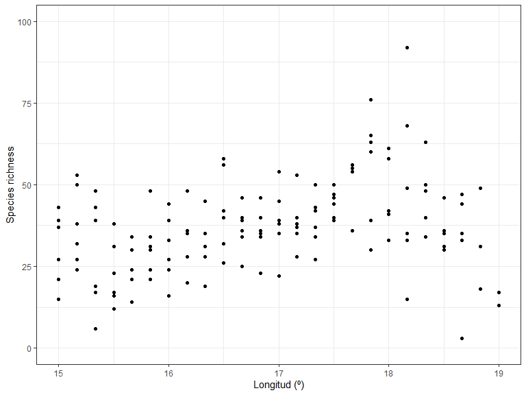
Species richness as a function of environment:
ggplot(xgridded, aes(meanTempWarmQuart, annPrec,
                     colour = richness)) +
  labs(x = "Mean temperature of warmest quarter (ºC)" ,
       y = "Annual precipitation (mm)",
       colour = "Species \nrichness") +
  scale_colour_distiller(palette = "Spectral") +
  geom_point(size=3) +
  theme_bw()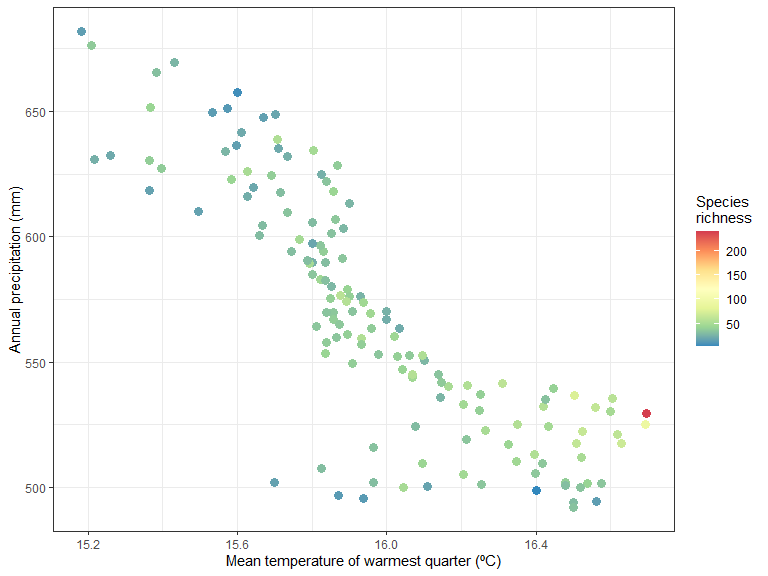
It seem like there is higher species richness in hottest areas.
How does the community composition change along the transect? Use clustering:
library(vegan)
## Bray-Curtis dissimilarity
D <- vegdist(xgridded[, sppcols], "bray")
## UPGMA clustering
cl <- hclust(D, method = "ave")
## plot the dendrogram
plot(cl)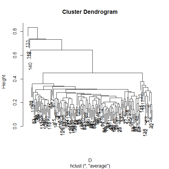
## extract group labels at the 10-group level
grp <- cutree(cl, 10)
grp <- sapply(grp, function(z)which(unique(grp) == z)) ## renumber groups
xgridded$grp <- as.factor(grp)
## plot
## colours for clusters
thiscol <- c("#1f77b4", "#ff7f0e", "#2ca02c", "#d62728", "#9467bd", "#8c564b",
             "#e377c2", "#7f7f7f", "#bcbd22", "#17becf")
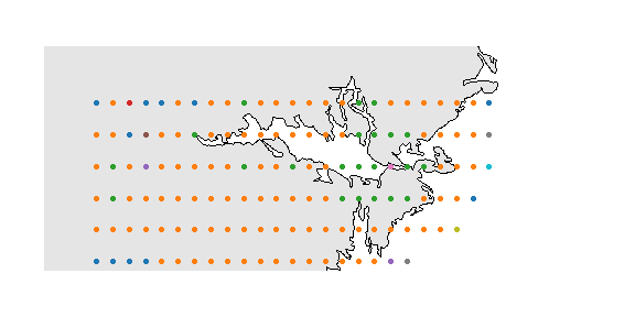
ggplot(xgridded, aes(longitude, latitude, colour = grp)) +
  labs(x = "Longitude", y = "Latitude", colour = "Group") +
  geom_point(size = 3) +
  scale_colour_manual(values = thiscol) +
  theme_bw()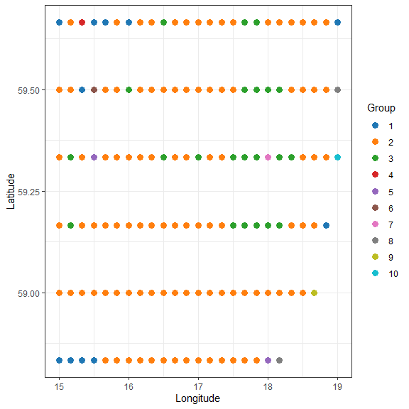
## or a slightly nicer map plot
library(maps)
library(mapdata)
oldpar <- par()
par(mar = c(1,1,0,0))
map("worldHires", "Sweden",
    xlim = c(14.5, 20), ylim = c(58.8, 59.95),
    col = "gray90", fill = TRUE)
with(xgridded, points(longitude, latitude,
                      pch = 21, col = thiscol[grp],
                      bg = thiscol[grp], cex = 0.75))
suppressWarnings(par(oldpar))